How to perform a one-sample t-test in R?

How to perform a one-sample t-test in R?. one-sample The t-test compares one sample’s mean to a known standard (or theoretical/hypothetical) mean.

One-sample t-tests can only be used when the data is normally distributed. The Shapiro-Wilk test can be used to verify this.

How to perform a one-sample t-test in R

Typical research questions are:

whether the sample mean (m) is the same as the theoretical mean ()?

whether the sample mean (m) is lower than the theoretical mean ()?

whether the sample mean (m) is higher than the theoretical mean ()?

In statistics, the analogous null hypothesis (H0) is defined as follows:

H0:m=μ
H0:m≤μ
H0:m≥μ

The following are the relevant alternative hypothesis (H1):

Ha:m≠μ (different)
Ha:m>μ (greater)
Ha:m<μ (less)

Keep in mind:

Two-tailed tests are used to test hypotheses 1.

One-tailed tests are used to test hypotheses 2 and 3.

One-sample t-test formula

The t-statistic can be determined using the following formula.

t=m−μ/(s/√n)

where,

m is the sample mean

n is the sample size

s is the sample standard deviation with n−1 degrees of freedom

μ is the theoretical value

For the degrees of freedom (df), we can compute the p-value equivalent to the absolute value of the t-test statistics (|t|): df=n1.

How should the results be interpreted?

We can reject the null hypothesis and accept the alternative hypothesis if the p-value is less than or equal to the significance level of 0.05. To put it another way, we’ve determined that the sample mean differs significantly from the theoretical mean.

In R, visualize your data and do a one-sample t-test.

Install the ggpubr R package to visualize data.

You can make R base graphs as explained here: Base graphs in R. For an easy ggplot2-based data visualization, we’ll use the ggpubr R tool.

install.packages("ggpubr")

One-sample t-test calculation in R

The R function t.test() can be used to do a one-sample t-test as follows.

t.test(x, mu = 0, alternative = "two.sided")

x: a numeric vector containing your data values

mu: the theoretical mean. Default is 0 but you can change it.

alternative: a different hypothesis “two.sided” (default), “greater” or “less” are all valid values.

Bring your data into R.

set.seed(123)
data <- data.frame(
  name = paste0(rep("P_", 10), 1:10),
  weight = round(rnorm(20, 30, 2), 1))

Examine your data the first ten rows of data should be printed.

head(data, 10)

name weight
1   P_1   28.9
2   P_2   29.5
3   P_3   33.1
4   P_4   30.1
5   P_5   30.3
6   P_6   33.4
7   P_7   30.9
8   P_8   27.5
9   P_9   28.6
10 P_10   29.1

Statistical weight summaries

summary(data$weight)

   Min. 1st Qu.  Median    Mean 3rd Qu.    Max.
  26.10   29.05   30.25   30.28   31.10   33.60

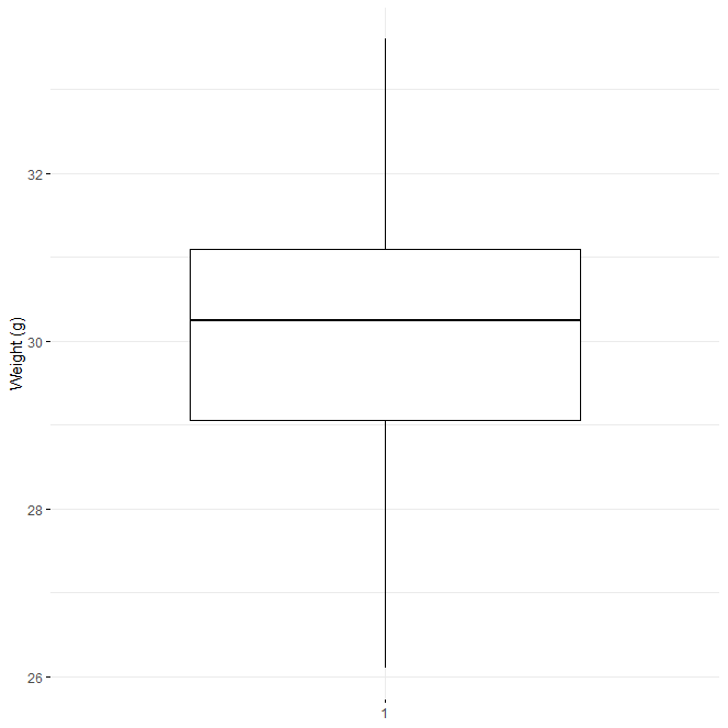
Use box plots to visualize your data.

library(ggpubr)
ggboxplot(data$weight,
          ylab = "Weight (g)", xlab = FALSE,
          ggtheme = theme_minimal())

One-Sample T-test for students in R

To check one-sample t-test assumptions, do a preliminary test.

Is this a representative sample? – No, because n is less than 30.

We must evaluate whether the data follow a normal distribution because the sample size is insufficient (less than 30, central limit theorem).

How do you check for normality?

Read this article: Test for Normal Distribution in R-Quick Guide

In a nutshell, the Shapiro-Wilk normality test and the normality plot can be used.

The Shapiro-Wilk test is used to determine whether the data are normally distributed.

Another possibility is that the data are not normally distributed.

shapiro.test(data$weight)

Shapiro-Wilk normality test
data:  data$weight
W = 0.97061, p-value = 0.7677

The p-value in the output is bigger than the significance level of 0.05, implying that the data distribution is not substantially different from normal. To put it another way, we can presume normality.

Q-Q plots are used to visually check the data for normality (quantile-quantile plots). The correlation between a particular sample and the normal distribution is depicted in a Q-Q plot.

Q-Q Plot

library("ggpubr")
ggqqplot(data$weight, ylab = "Men's weight",
         ggtheme = theme_minimal())

One-Sample Student’s T-test in R

We conclude that the data may come from normal distributions based on the normality plots.

Note that if the data are not normally distributed, the non-parametric one-sample Wilcoxon rank test is advised.

Make a one-sample t-test.

If the average weight of the mice differs from 22g (two-tailed test), we want to know.

One-sample t-test

res <- t.test(data$weight, mu = 22)
res

One Sample t-test
data:  data$weight
t = 19.146, df = 19, p-value = 7.031e-14
alternative hypothesis: true mean is not equal to 22
95 percent confidence interval:
 29.37483 31.18517
sample estimates:
mean of x
    30.28

If you wish to see if mice mean weight is less than 22g (one-tailed test), type:

t.test(data$weight, mu = 22,
              alternative = "less")

One Sample t-test alternative=less

data:  data$weight
t = 19.146, df = 19, p-value = 1
alternative hypothesis: true mean is less than 22
95 percent confidence interval:
    -Inf 31.0278
sample estimates:
mean of x
    30.28

Alternatively, type this to see if the mean weight of mice is larger than 22g (one-tailed test):

t.test(data$weight, mu = 22,
              alternative = "greater")

One Sample t-test alternative=greater

data:  data$weight
t = 19.146, df = 19, p-value = 3.516e-14
alternative hypothesis: true mean is greater than 22
95 percent confidence interval:
 29.5322     Inf
sample estimates:
mean of x
    30.28

Interpretation of the result

The test’s p-value is less than the significance level of alpha = 0.05. We can deduce that the mice’s average weight is significantly different from 22g.

The values returned by the t.test() function can be accessed.

The t.test() function returns a list with the following components:

statistic: the t-test statistic’s value

parameter: the t-test statistics degrees of freedom

p.value: the p-value for the test

conf.int: a confidence interval for the mean appropriate to the specified alternative hypothesis.

estimate: the difference in means between the two groups being compared (in the case of an independent t-test) (in the case of paired t-test).

The R code to use to acquire these values has the following format: