One-Sample Wilcoxon Signed Rank Test in R?, When the data cannot be assumed to be normally distributed, the one-sample Wilcoxon signed-rank test is a non-parametric alternative to the one-sample t-test.
It’s used to see if the sample’s median is the same as a known standard value (i.e. theoretical value).
The data should be symmetrically distributed around the median. In other words, the number of numbers above and below the median should be nearly equal.
Common research questions include:
- whether the sample’s median (m) equals the theoretical value (m0)?
2. whether the sample’s median (m) lower than the theoretical value (m0)?
3. whether the sample’s median (m) higher than the theoretical value (m0)?
In statistics, the analogous null hypothesis (H0) is defined as follows:
H0:m=m0
H0:m≤m0
H0:m≥m0
The following are the relevant alternative hypothesis (H1):
Ha:m≠m0 (different)
Ha:m>m0 (greater)
Ha:m<m0 (less)
Note that:
Two-tailed tests are used to test hypotheses 1.
One-tailed tests are used to test hypotheses 2 and 3.
Visualize your data and do one-sample calculations. Install the ggpubr R package for data visualization to perform the Wilcoxon test in R.
R base graphs can be created as explained here: R base graphs. For easy ggplot2-based data visualization,
we’ll use the ggpubr R tool. install from CRAN as follow:
install.packages("ggpubr")
Wilcoxon one-sample test with the R function
The R function wilcox.test() can be used to do a one-sample Wilcoxon test as follows.
wilcox.test(x, mu = 0, alternative = "two.sided")
x: a numeric vector containing your data values
mu: the theoretical value of mean/median The default value is zero, but you can modify it.
alternative: the opposite hypothesis “two.sided” (default), “greater” or “less” are all valid values.
We’ll use a data collection including the weights of ten mice as an example.
If the mice’s median weight differs from 22g, we’d like to know.
set.seed(123)
data <- data.frame(
  name = paste0(rep("P_", 10), 1:10),
  weight = round(rnorm(20, 30, 2), 1))
Let’s print the first 10 rows of the data
head(data, 10)
name weight
1   P_1   28.9
2   P_2   29.5
3   P_3   33.1
4   P_4   30.1
5   P_5   30.3
6   P_6   33.4
7   P_7   30.9
8   P_8   27.5
9   P_9   28.6
10 P_10   29.1
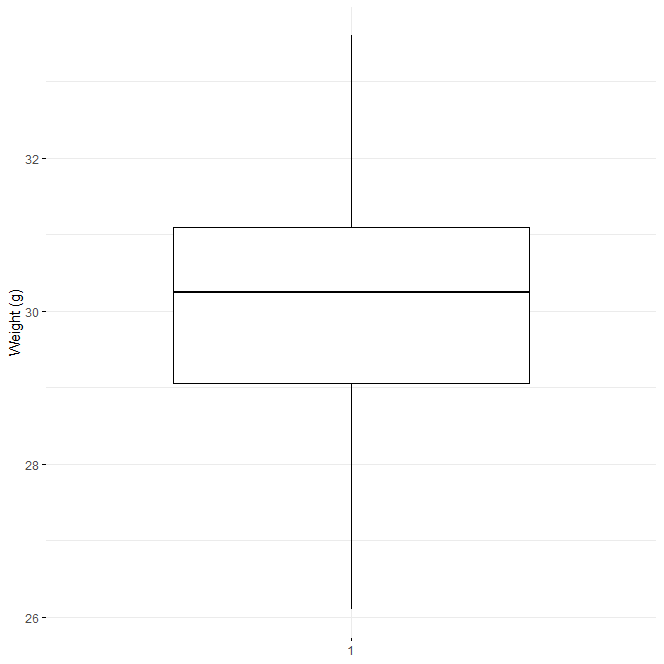
Statistical summaries of weight
summary(data$weight)
  Min. 1st Qu.  Median    Mean 3rd Qu.    Max.
  26.10   29.05   30.25   30.28   31.10   33.60
Minimum: the lowest value
The first quartile: Only 25% of the values are lower than this.
The median is the middle value. Half of the readings are lower, while the other half are higher.
The third quartile: The majority of the values are higher.
Maximum: the highest value
Use box plots to visualize your data.
library(ggpubr)
ggboxplot(data$weight,
          ylab = "Weight (g)", xlab = FALSE,
         ggtheme = theme_minimal())

In R, compute a one-sample Wilcoxon signed-rank test.
If the average weight of the mice differs from 22g (two-tailed test), we want to know.
# One-sample Wilcoxon test
res <- wilcox.test(data$weight, mu = 22)
res
Wilcoxon signed-rank test with continuity correction
data:  data$weight
V = 210, p-value = 9.542e-05
alternative hypothesis: true location is not equal to 22
Now we can print only the p-value
res$p.value
9.542331e-05
The test’s p-value is less than the significance level of alpha = 0.05. We can rule out the null hypothesis and infer that the mice’s average weight differs significantly from 22g.
Keep in mind:
Type this if you wish to see if the median weight of mice is less than 22g (one-tailed test):
wilcox.test(data$weight, mu = 22,
              alternative = "less")
Wilcoxon signed-rank test with continuity correction
data:  data$weight
V = 210, p-value = 1
alternative hypothesis: true location is less than 22
Alternatively, type this to see if the median weight of mice is larger than 22g (one-tailed test).
Statistical test assumptions and requirements
wilcox.test(data$weight, mu = 22,
              alternative = "greater")
Wilcoxon signed-rank test with continuity correction
data:  data$weight
V = 210, p-value = 4.771e-05
alternative hypothesis: true location is greater than 22


