


Dealing With Missing Values in R, one of the issues is that when you have a large matrix of data and some of the columns have a few missing values, it might be difficult to work with.
Checking Missing Values in R – (datasciencetut.com)
You won’t be able to perform a lot of multivariate or bivariate studies. As a result, we frequently want to be able to substitute missing values for them known as data imputation.
So that’s all we are going to say about it. The data imputation, necessitates the installation of a package, thus the package.
So there’s a package called a mice, you should enter the below code if not installed the package.
install.packages("mice")
Now, in the package, it has some examples so here we have
library(mice)
and we’ll have data, therefore we’ll use mammal sleep data as an example. Then you can inquire about mammal sleep data. Let’s have a look at mammalsleep.
?mammalseep
What does the data on mammal sleep tell us?
We have a few animal species. Body mass index, brain mass index, slow-wave sleep, paradoxical sleep, total sleep, maximum lifespan, gestation time, predation index, sleep exposure index, and overall danger index is all factors to consider.
So, now that we have the data, we can examine it. So mammalsleep, just to tell you how many rows and columns, it’s a little bigger than what would fit on the screen.
head(mammalsleep)
So, because there are 62 rows, let’s start at the beginning.
you’ll see the first few observations.
                                  species       bw    brw sws  ps   ts  mls  gt pi sei odi
1          African elephant 6654.000 5712.0  NA  NA  3.3 38.6 645  3   5   3
2 African giant pouched rat    1.000    6.6 6.3 2.0  8.3  4.5  42  3   1   3
3                Arctic Fox    3.385   44.5  NA  NA 12.5 14.0  60  1   1   1
4    Arctic ground squirrel    0.920    5.7  NA  NA 16.5   NA  25  5   2   3
5            Asian elephant 2547.000 4603.0 2.1 1.8  3.9 69.0 624  3   5   4
6                    Baboon   10.550  179.5 9.1 0.7  9.8 27.0 180  4   4   4
So far, we’ve established the species, and we’ll begin with the African elephant. Various mammals descend here, and body weight is highly variable, as is evidenced by several of the data related to sleep.
So, for example, the slow-wave sleep measurement has not been done because it is unlikely to be practical to do so in the wild, on an African elephant, example.
As a result, the missing measures are identified. They are instantly recognizable.
You’ve got NA, NA, NA, and so on.
dim(mammalsleep)
[1] 62 11
So the function which tells me how many missing variables there are is called nic().
nic(mammalsleep)
And now it says there are 20 of us. As a result, nic() is the number of the absence of clarity.
Is there at least one NA in that row? So the number of incomplete cases is tested across every row.
As a result, we can see that 20 of the 62 examples are missing.
When we removed all of the data with missing variables, we were left with 42 instead of 62.
That accounts for almost a third of the data. Now, ignoring anything about those observations can be destructive to the entire study, so we have the means to accomplish what’s known as imputation.
Now, the way it works is that you have to look for these missing data in some method. So, in mice, we have a function that informs us where they are.
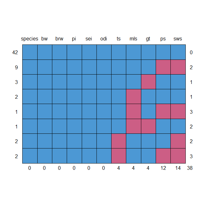
So we have md.pattern, which tells me about the missing variable pattern in mammalsleep.
md.pattern(mammalsleep)
 species bw brw pi sei odi ts mls gt ps sws
42       1  1   1  1   1   1  1   1  1  1   1  0
9        1  1   1  1   1   1  1   1  1  0   0  2
3        1  1   1  1   1   1  1   1  0  1   1  1
2        1  1   1  1   1   1  1   0  1  1   1  1
1        1  1   1  1   1   1  1   0  1  0   0  3
1        1  1   1  1   1   1  1   0  0  1   1  2
2        1  1   1  1   1   1  0   1  1  1   0  2
2        1  1   1  1   1   1  0   1  1  0   0  3
         0  0   0  0   0   0  4   4  4 12  14 38
So we have 42 observations with no missing data, indicating that this is, in some ways, counting the entire cases.
As a result, we’ve arrived at number 42, where you’ll find entire cases on everything. We have two mls files that are missing, as well as one gt file that is missing.
What exactly are we on the lookout for?
Why do we pay attention to these patterns?
When trying to impute data, you shouldn’t have too many blocks of variables that are all missing simultaneously.
So the maximum you have is three observations for which we have ts, ps, and these are the sleeping variables that are present.
We also have several with the mls, ps, and sws loaded. As a result, the patterns aren’t overly blocky.
And that’s what you’re looking for when you’re trying to figure out what’s lacking. If they’re too many in blocks, we refer to them as systematic patterns, and we refer to them as missing not at random, or MNAR, as opposed to missing at random, or MCAR.
And so that’s something you look for when you’re just trying to figure out if you can impute them.
And so, with the help of the function mice, you should look into the actual imputation; they have a variety of methods for doing so, and they show you how to accomplish it just by using the mice function.
So we could perform imp, which stands for imputed data, and mice(mammalsleep), which is an iterative procedure that takes care of obtaining local averages, and this is because the lines emerge one by one.
imp<-mice(mammalsleep)
iter imp variable
  1   1  sws*  ps*  ts*  mls*  gt*
  1   2  sws*  ps*  ts*  mls*  gt*
  1   3  sws*  ps*  ts*  mls*  gt*
  4   1  sws*  ps*  ts*  mls*  gt*
   .....................................................
As a result, it makes an educated guess at a reasonable value.
And now, if I look at the values returned by head(imp), you can see the results.
So, for example, for sws, you guessed that part of the values throughout a number of permutations are imputed, and this is the original data.
So we have the original data and the data that is missing. So there was the $data and the $call.
As you can see, we have the actual data that the imputation function returns, as well as the imputed values for when it happens, whether as most of the imputation.
This is the total number of steps it took. Will catch up with some other interesting posts soon…

